1 Basics Of Filtering

Before looking at how Kalman filters worked basic recursive filters were tested. Later the performance between these and the Kalman filter will be compared. The purpose of a filter is to consider measurements and use these to form an estimate of the true state.

The true state \(x_k\) (at time \(t_k\)) is a column vector describing the system. The state estimate, \(\hat{x}_k\) (at time \(t_k\)), is the estimate of the state based on the measurements \(z_k\) (at time \(t_k\)), which are corrupted by noise.

1.1 Average filters

For a signal where \(x_k\) is constant, e.g. calculating the output from a battery, computing the mean is a reasonable way to determine \(\hat{x}_k\). The average is computed as:

(1)\[\hat{x}_k = \frac{z_1+z_2+z_3+...+z_k}{k}\]

In this case \(\hat{x}_k\) is the average. However \(\hat{x}_k\) needs to be computed at every time-step, (1) isn’t going to be very efficient to compute. Written in a more computationally efficient form:

(2)\[\hat{x}_k = \left(\frac{k-1}{k}\right)\hat{x}_{k-1} + \frac{z_k}{k}\]

Let \(\alpha = \frac{k-1}{k}\), (2) can be rewritten as:

(3)\[\hat{x}_k = \alpha \hat{x}_{k-1} + (1 - \alpha) z_k\]

This will be referred to as the recursive average filter. The code for this filter can be found in github. The programme is made up from 3 files: GetVolt.py, RcsAvgFilter.py and Test.py. The first file generates a noisy signal, the second contains the filter and the third runs the filter on the generated signal.

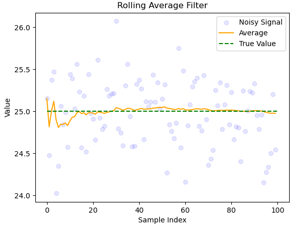
Fig. 1 A noisy signal with mean 25 and standard deviation 0.5, fitted with a moving average filter.

The filter is efficient and converges to the correct value very quickly. Due to random variation the filter fluctuates around the correct value. The average filter is very good when \(\hat{x}_k\) is constant, however it won’t converge to a changing signal.

1.2 Moving Average filters

The moving average is used to remove noise over a constantly varying signal. Here \(\hat{x}_k\) represents the moving average at time \(t_k\) and \(n\) represents the window size which is a parameter to be tuned. The moving average can be written as:

(4)\[\hat{x}_k = \frac{z_{k-n+1} + z_{k-n+2}+...+z_k}{n}\]

\(\hat{x}_k\) can be written recursively using the previous estimate \(\hat{x}_{k-1}\) and the new measurement \(z_k\):

(5)\[\hat{x}_k = \hat{x}_{k-1} + \frac{z_n - z_{k-n}}{n} \]

for more efficient computation. The code for the following graphs can be found in github. The programme is made up from 3 files: GenTestSig.py, MovAvgFilter.py and Main.py. The first file generates a signal (the true signal) which is a combination of 3 \(\sin\) waves and then adds random gaussian noise to this signal, the noisy signal. The second contains the filter algorithm which will be used to fit the noisy signal and the third runs the filter on the generated signal.

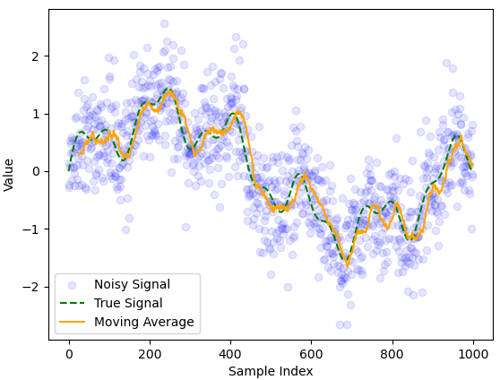
Fig. 2 Moving average filter applied to a noisy signal with \(n = 25\).

The moving average lags behind the true signal but has roughly the right shape. This is expected as the moving average relies on previous estimates.

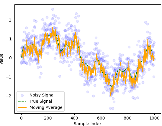
Fig. 3 Moving average filter applied to a noisy signal with \(n=5\).

In this example the delay is smaller but less noise is removed. There is a tradeoff between noise reduction and minimizing delay limiting the accuracy of the moving average filter.

1.3 Exponential Moving Average filter (Low Pass)

All terms in (4) have equal weighting (\(1/n\)), however it makes more sense to give more recent terms a larger weighting, this should help minimize delay whilst preserving the smoothing effect. A result of this is it allows low frequencies to pass through but filters out high frequencies. Noise is usually high frequency. Below is an example of a first order exponential moving average, low pass filter (EMALPF):

(6)\[\hat{x}_k = \alpha \hat{x}_{k-1} + (1 - \alpha) z_k \quad 0<\alpha<1\]

Looks similar to (3) except here \(\alpha\) is a parameter to be tuned. It is also true that:

(7)\[\hat{x}_{k-1} = \alpha \hat{x}_{k-2} + (1 - \alpha) z_{k-1} \quad 0<\alpha<1\]

Combining these equations helps to overcome some problems associated with the moving average since more distant terms disappear exponentially quickly:

(8)\[\hat{x}_k = \alpha^2 \hat{x}_{k-2} + \alpha(1-\alpha) z_{k-1} + (1-\alpha)z_k \quad 0<\alpha<1\]

Due to the restriction on alpha larger \(n\) means greater weighting on \(\hat{x}_n\) since \(\alpha(1-\alpha)\leq 1-\alpha\). Previous data gets weighted exponentially less.

The code for this section can be found in github. Similarly to the other two examples the code is made up of 3 files: GenTestSig.py, LowPassFilter.py and Main.py. The first file generates a signal (the true signal) which is again a combination of 3 \(\sin\) waves and then adds random gaussian noise to this signal, the noisy signal. The second contains the filter algorithm which will be used to fit the noisy signal and the third runs the filter on the generated signal.

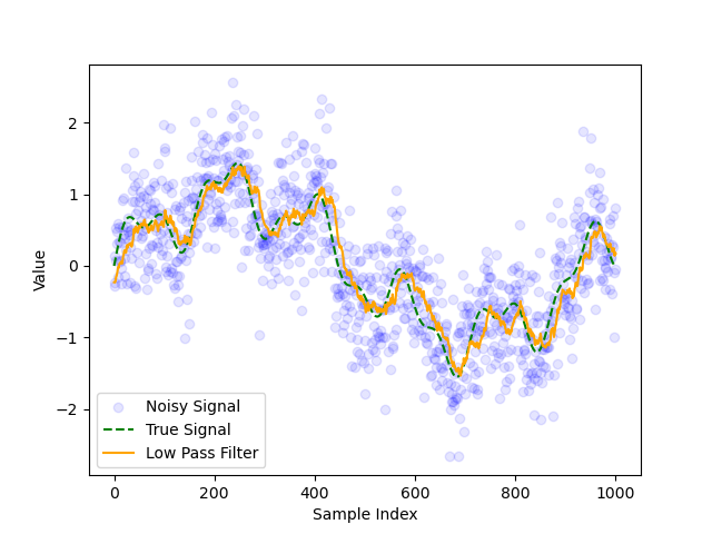
Fig. 4 Figure 3.1: EMALPF with optimized \(\alpha = 0.93\) (visually).

The low pass filter has a smaller delay compared to the moving average filter, but was nosier. This makes sense as the moving average filter gives equal weight to all previous estimates, so noisy measurements will have a smaller effect on the fit.

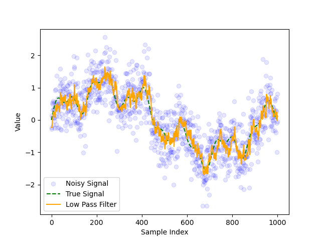
Fig. 5 Figure 3.2: Low pass filter with \(\alpha = 0.8\).

Here the delay is less significant but the filter doesn’t remove as much noise compared to Fig. 4, since the weighting on previous estimates is smaller.

Fig. 6 Figure 3.3: Low pass filter with \(\alpha = 0.97\).

Here the delay is more significant since previous results are given larger weightings. The choice of \(\alpha\) represents a tradeoff between a noisy signal and a delayed signal, which means its difficult to find optimal \(\alpha\).

1.4 Exponential Moving Average Filter (High Pass)

An exponential moving average high pass filter (EMAHPF) works by subtracting the EMALPF \(\hat{x}^{LP}_k\) from \(z_k\). This corresponds to removing the low frequencies from the signal. The high pass filter estimates the state \(\hat{x}^{HP}_k\) as:

(9)\[\hat{x}_k^{HP} = z_k - \hat{x}^{LP}_k \]

Subbing in (6) gives:

(10)\[\hat{x}_k^{HP} = \alpha (\hat{x}^{LP}_{k-1} + z_k)\]

Then subbing (9) rearranged into (10) gives:

(11)\[\hat{x}_k^{HP} = \hat{x}_{k-1}^{HP} + z_k - z_{k-1}\]

Which is the recursive formula for the EMAHPF. These are useful for removing low frequency background noise, such as integration drift.

1.5 Summary

The above are examples of passive filters as they filter data without using feedback from a physical model. Kalman filters are active filters which compare measurements with feedback to determine an improved estimate of the state.