8 Experiment: Quantitative Comparison of Kalman Filter Performance

Using two sensors (magnetometer and gyroscope), four filters (a high pass, a low pass, a polynomial fitting and the kalman filter) were used to calculate estimates for the yaw angle, \(\psi\), of a mobile phone. The results were compared to the data from the phones in built filter. The experiment involved two tests designed to see how the filters perform over a single frequency then a range of frequencies. In the first part of the experiment the phone oscillated with high frequency which the parameters were tuned, to test how the filters performed at a single frequency. The second part of the experiment the phone completed a full rotation at a low frequency without the parameters being re-tuned, to see how the filters responded when not tuned to a specific frequency.

8.1 Implementation

Data was recorded using the sensor logger app allowing the phone to function as a 9-axis IMU. Only \(\psi\) was measured so only gyroscope and magnetometer data were necessary. The correction measurement was calculated using the magnetometer data \(m_x\) and \(m_y\). \(m_z\) wasn’t required as the IMU was assumed to be in the plane perpendicular to the gravity vector, so didn’t need to be corrected. \(\psi\) was determined using (53).

The gyroscope data was integrated using the euler method:

(55)\[\psi_k \approx \psi_{k-1} + \omega_k \Delta t\]

This time \(\omega_k\) is the gyroscope measurement of angular velocity at time \(k\) in the \(z\) direction. This formed the prediction measurement. The form required by the Kalman filter is \(\hat{x}^-_k = A\hat{x}_{k-1} + Bu_k\). So \(A = 1\) and \(B = dt\) and \(u_k = \omega_k\). The state to measurement matrix \(H = 1\) since \(z_k\) and \(\hat{x}_k\) are both the yaw angle.

The code for this section can be found in github. The programme comprises of one file Main.py. Each of the filters is written as a separate function and can be analyzed using the AnalysePhone class, which contains methods to generate interactive plots.

8.2 Filters

The following filters were compared as well as unfiltered data from the gyroscope and the magnetometer:

Kalman Filter (KF): A standard Kalman filter which fused data from the magnetometer with gyroscope data with a constant process noise covariance and measurement noise covariance. The tuning parameters were:

• \(Q\): Process noise covariance.

• \(R^m\): Measurement noise covariance for the magnetometer measurements.

• \(R^g\): Measurement noise covariance for the gyroscope measurements.

Exponential Moving Average Low Pass Filter (EMAHPF): Was applied to the magnetometer data where the Where \(\alpha^{HP}\) is the tuning parameter, to reduce noise.

Exponential Moving Average High Pass Filter (EMAHPF): Was applied to gyroscope data to cutout integration drift (low frequency). \(\alpha^{LP}\) was the tuning parameter.

Savitzky-Golay Filter (SGF): Was applied to the magnetometer data to help mitigate random noise. It has the following parameters:

• \(W\): The length of the filter window.

• \(\mathbb{O}\): The order of the polynomial used to fit the samples. The SGF works by fitting a polynomial of order \(\mathbb{O}\) to a window of length \(W\). The center of the window is the fitted value.

8.3 Results

High frequency oscillation test

The phone was initially held in a fixed position for around 5 seconds then oscillated at a high frequency for around \(20\) s, each of the filters was tuned to optimise the fit.

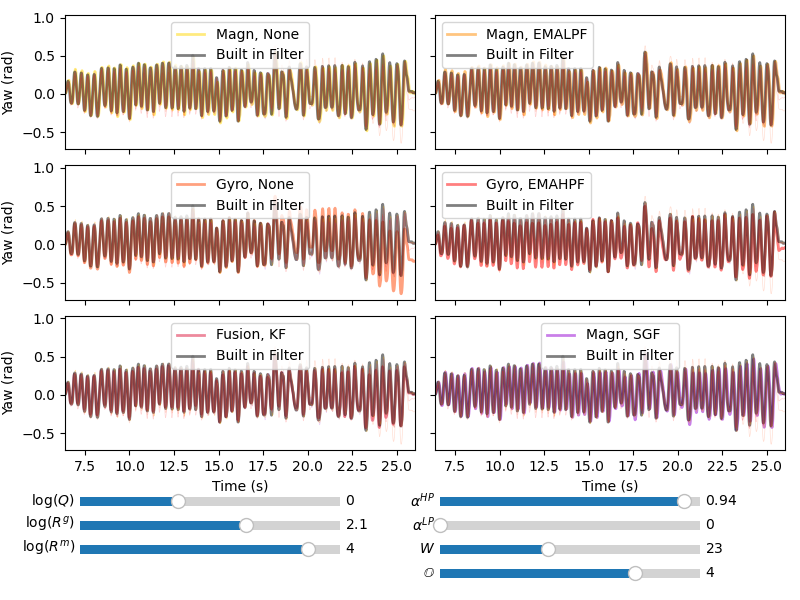
Fig. 36 Shows the signal used and gives an overview of the results and compares the phones own filters against the filters described above. Tuning parameters were set below.

Fig. 36 shows integration drift is visible in the unfiltered gyroscope data. But all other filters seem to be a good fit from a distance.

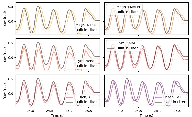
Fig. 37 Zoomed in view of the final few oscillations of the high frequency oscillation experiment with a visually optimized fit.

Fig. 37 shows the there is integration drift from the unfiltered gyroscope data but not with the EMAHPF since the drift is low-frequency. The magnetometer measurments are lagging behind the true signal which also effects the EMALPF and SGF. Surprisingly the Kalman filter isn’t lagged as it relies heavily on the gyroscope measurements. The Kalman filter assumes a large amount of noise in the magnetometer, \(R_m\), two orders of magnitude larger than \(R_g\). There is also a small amount of linear process noise.

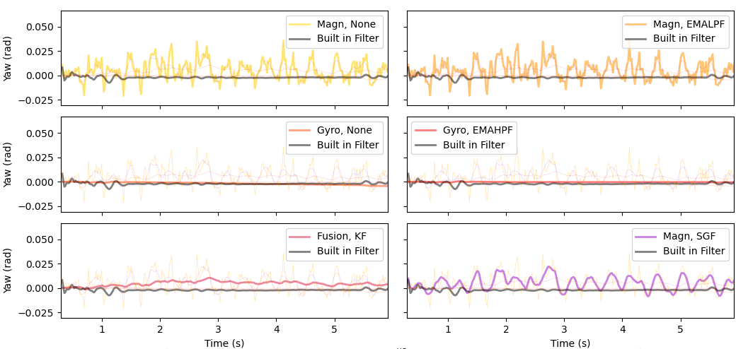
Fig. 38 Zoomed in view of the flat proportion of the graph, at the beginning.

Fig. 38 shows the noisiest sensor is the magnetometer. The SGF reduces some of this noise. The EMALPF actually made the fit worse since the noise from the magnetometer was significantly less significant than its lag, which applying a low-pass filter actually worsened.

Note

\(R^2\) measures the pattern-matching ability of the filter and is sensitive to phase shifts. MSE (mean squared error) measures absolute accuracy and heavily penalizes large errors due to squaring.

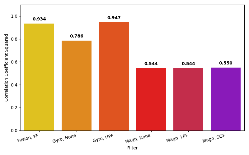
Fig. 39 Correlation coefficient squared, \(R^2\) for each of the filters against the phones built in filter.

None of the measurements using the magnetometer perform well. The best of the magnetometer measurements is the SGF, as it removes a small amount of noise and doesn’t cause significant lag. Fig. 39 suggests that the EMALPF fits the shape the best on the gyro data than the fused KF did, likely a result of lagging magnetometer data which wasn’t corrected for.

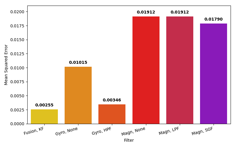
Fig. 40 MSE for each of the filters against the phones builtin filter for the first test.

Conversely Fig. 40 suggests that KF has a more accurate fit. This suggests that EMALPF fits the shape of the data better than KF but KF is on average more accurate.

Low frequency rotations test

The phone was held still for around \(8\)s and then was rotated a full circle over the space of the next \(15\)s. The tuning parameters for this experiment are those given in Fig. 36.

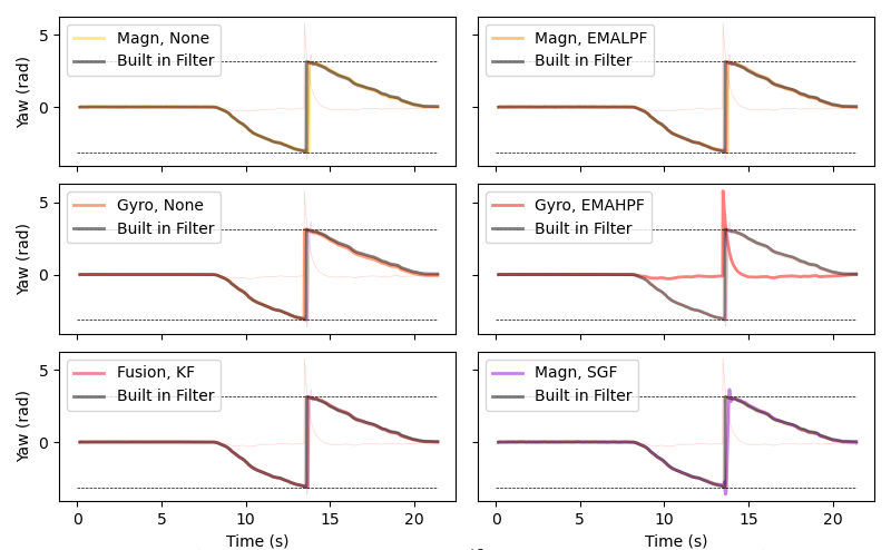
Fig. 41 Comparison of the phones own filters against the filters described above. With tuning parameters the same as Fig. 36.

Fig. 41 shows that all filters are a good fit for the data except the EMAHPF which filters out the low frequencies even if they are not related to noise, in this case the slow rotation.

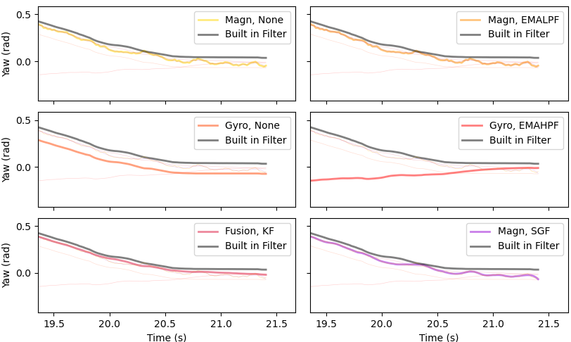
Fig. 42 Zooming in on the last couple of seconds of Fig. 41.

Fig. 42 shows that there has been some drift from all the filters away from the true yaw. But the Kalman filter is closest to the true value. As expected the gyro produces a much smoother fit compared to the magnetometer. Applying a low pass filter to the magnetometer data would make the fit for gyro data better but this would result in some of the higher frequencies being lost which will result in a worse fit for the first test.

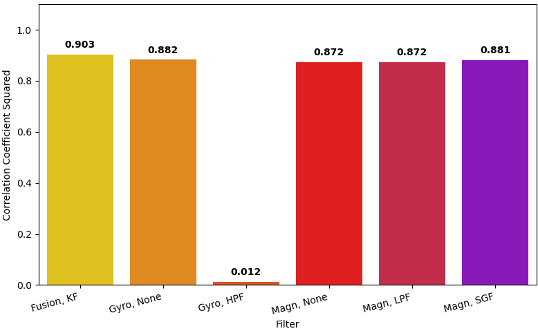
Fig. 43 \(R^2\) for each of the filters against the phones built in filter.

Fig. 43 shows the Kalman filter produced the best fit as did all the other filters except the EMAHPF which had a very poor fit. The magnetometer data gave a much better fit in these examples compared to the previous test as the oscillations are significantly slower, the lag is less significant. In general the second signal is much easier to fit than the first.

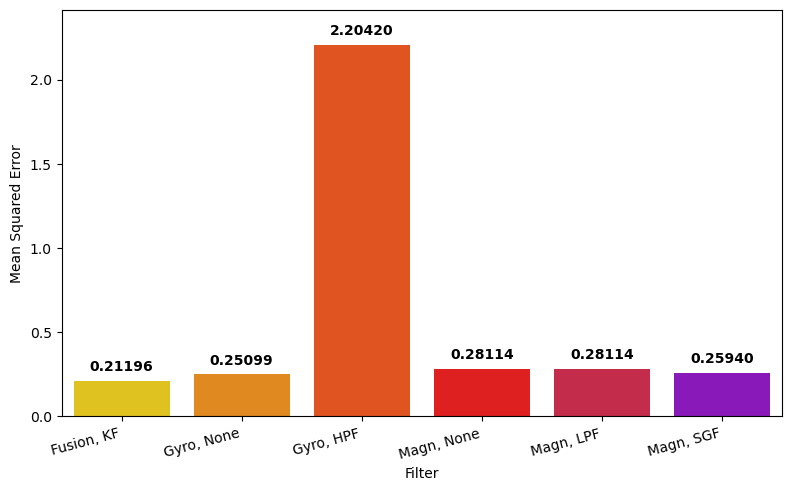
Fig. 44 MSE for each of the filters against the phones builtin filter for the second test.

Fig. 44 indicates the same as Fig. 43, the Kalman filter still provides a marginally better fit than the other filters. The EMAHPF, which had the best fit in the first test now has by far the worst fit as discussed earlier.

8.4 Conclusion

Frequency based filters, like the EMAHPF and EMALPF work well for signals which are oscillating at a constant or near constant frequency, especially when there is only one sensor available. However they work less well for a signal made up from a range of different frequencies, like real world motion. Kalman filters work well in this situation as the combination of measurements minimizes noise from both sensors (which are subject to different types of noise) to achieve a reasonably accurate state estimate, without ignoring any specific frequency data. The parameters of the KF are independent of frequency whereas the EMAHPF and EMALPF have frequency dependent tuning parameters.