5 Example: Attitude using a gyroscope and accelerometer

This section calculating the attitude of an object (yaw-pitch-roll), using real world sensor data. Firstly using the gyroscope to measure the angular velocity and then using Euler’s method for integration to obtain a prediction for the attitude, then improving this using a kalman filter, however this estimate drifts and becomes less accurate over time. To reduce drift accelerometer is used and the Kalman filter fuses data from the accelerometer and gyroscope.

The code for this section can be found in here. The code is broken up into 3 files: Test.py which runs the filter and plots the results; AdvKalman.py which contains the kalman filter algorithm; and Integrate.py which contains the integration algorithm which calculates the attitude without the kalman filter.

This example and raw data was provided by Dr Shane Ross a link to the video can be found here.

5.1 Euler’s method

Using gyroscope (measures angular velocity, \(\boldsymbol{\omega}\)) and knowing the attitude at \(t_0\) it is possible to determine the attitude of a craft at \(t_k\). The relationship between the body angular velocity \(\boldsymbol{\omega} = (\omega_1, \omega_2, \omega_3)\) and the time derivatives of the Euler angles \(\boldsymbol{\alpha} = (\psi, \theta, \phi)\) in the 3-2-1 (yaw-pitch-roll) sequence is given by the kinematic differential equation (KDE) below:

\(\phi\), \(\theta\) and \(\psi\) are euler angles that describe the orientation of the object in space. Whereas \(\omega_1\), \(\omega_2\), \(\omega_3\) are rates of rotation i.e. roll rate pitch rate and yaw rate.

\(\psi\), yaw: measures the rotation around the vertical (z) axis e.g. turning your head left and right in a “no” motion

\(\theta\), pitch: measures the rotation around the sided-to-side (y) axis e.g. nodding your head up and down in a “yes” motion.

\(\phi\), roll: rotation around the front-to-back (x) axis. E.g tilting your head to touch your ear to your shoulder.

The Euler angle rates \(\dot{\phi}\), \(\dot{\theta}\), \(\dot{\psi}\) are not the same as body angular rates because the orientation of the body axes changes as the object rotates.

(37)\[\begin{split}\begin{bmatrix} \dot{\psi} \\ \dot{\theta} \\ \dot{\phi} \end{bmatrix} = \frac{1}{\cos{\theta}}\begin{bmatrix} 0 & \sin\phi & \cos\phi \\ 0 & \cos\phi\cos\theta & -\sin\phi\cos\theta \\ \cos\theta & \sin\phi\sin\theta & \cos\phi \sin\theta \end{bmatrix} \begin{bmatrix} \omega_1 \\ \omega_2 \\ \omega_3 \end{bmatrix}\end{split}\]

Or more simply :

(38)\[\dot{\boldsymbol{\alpha}} = \Phi(\boldsymbol{\alpha}) {\boldsymbol{\omega}}\]

where \(\Phi(\boldsymbol{\alpha}) = \frac{1}{\cos{\boldsymbol{\theta}}}\begin{bmatrix} 0 & \sin\phi & \cos\phi \\ 0 & \cos\phi\cos\theta & -\sin\phi\cos\theta \\ \cos\theta & \sin\phi\sin\theta & \cos\phi \sin\theta \end{bmatrix}\)

The rates of rotation (provided by the gyroscope) are integrated step by step to predict the craft’s attitude at any later time \(t_k\):

(39)\[\boldsymbol{\alpha}_{k+1} \approx \boldsymbol{\alpha}_k + \dot{\boldsymbol{\alpha}}_k \Delta t\]

Subbing the relationship between \(\dot{\alpha}_k\) and \(\omega\) (38) into the update rule (39) gives:

(40)\[\boldsymbol{\alpha}_{k+1} \approx \boldsymbol{\alpha}_{k} + \Phi(\boldsymbol{\alpha}_k) \boldsymbol{\omega}_k \Delta t\]

where \(\Delta t = t_k - t_{k-1}\).

why use \(\approx\) not \(=\)

There is a small error associated with discretizing \(dt\) since \(\Delta t\) isn’t infinitesimally small. This is negligible term to term but over a large number of terms such as in this example the error accumulates and causes drift.

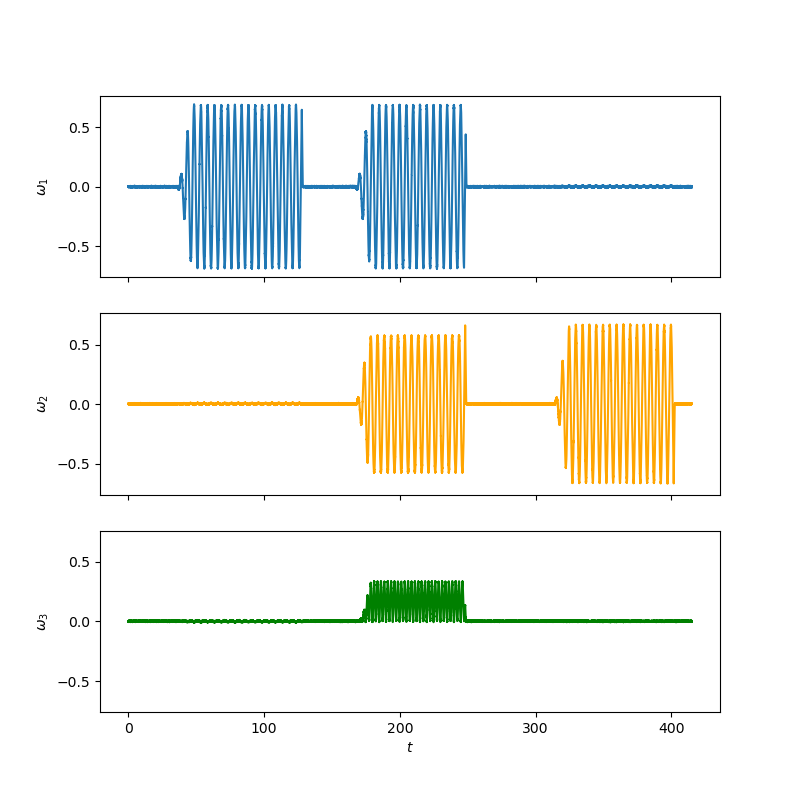
Fig. 16 Calibration signal involved shaking the device in just the \(\omega_1\) direction then pausing and shaking the device in the \(\omega_1\) and \(\omega_2\) directions before pausing again and shaking the device in the \(\omega_3\). The observed motion in the \(\omega_3\) direction was erroneous. View in Github

Using the calibration data in Fig. 16 and knowing the initial attitude (40) can be used to estimate the attitude over time:

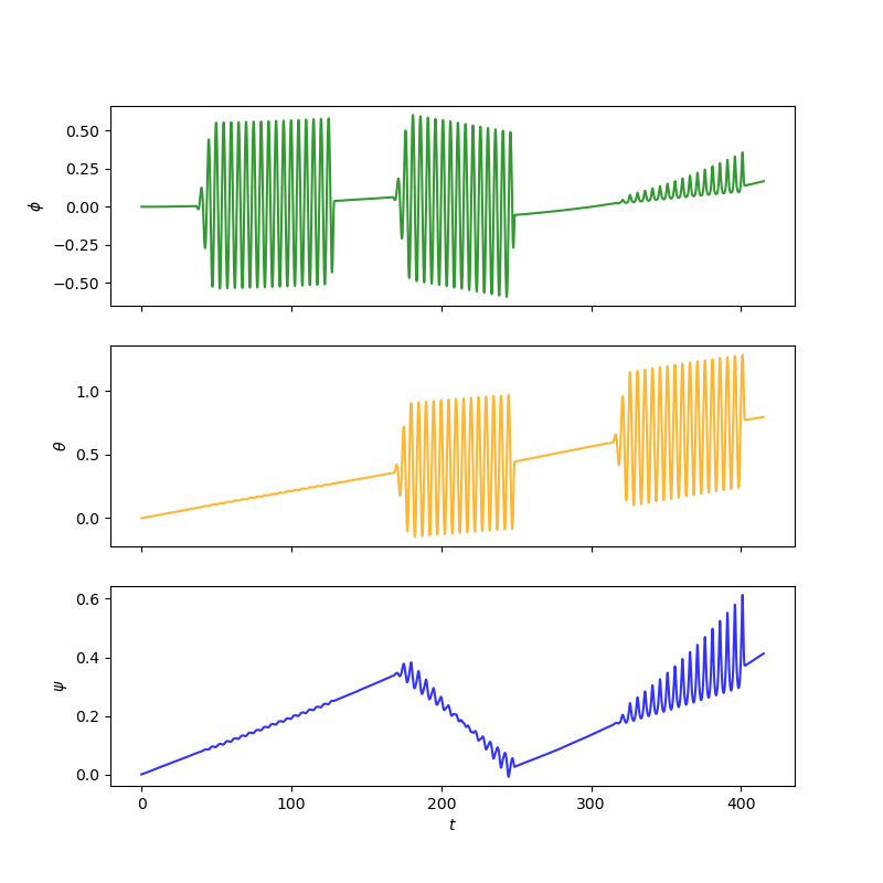
Fig. 17 \(\boldsymbol{\alpha}_k\) in each direction plotted against \(t_k\). View in Github

Overall the attitude \(\boldsymbol{\alpha}_k\) follows the generic shape of the true attude. The drift is least significant in the \(\phi\) direction but was predicting oscillations in the third part of the calibration even though there were no oscillations in the \(\omega_3\) direction at that time, and the drift also changes direction randomly. Drift was most pronounced in the \(\theta\) direction therefore the estimate becomes less accurate over time.

Drift is caused by the error associated with the numerical integration accumulating over time. The unexpected oscillations are likely from the gyroscope being sensetive to noise. Furthermore the oscillations could be coupled meaning small oscillations in one direction can be amplified in another.

5.2 Kalman filters

The model can be improved using a Kalman filter. However there is a problem as its not possible to put our update equation (40) into the form required for the kalman filter (32). To fix this the attitude was instead written in quaternions.

Tip

Use Euler parameters:

(41)\[ \begin{align}\begin{aligned}\beta_0 = \sin\frac{\phi}{2}\sin\frac{\theta}{2}\sin\frac{\psi}{2} + \cos\frac{\phi}{2}\cos\frac{\theta}{2}\cos\frac{\psi}{2}\\\beta_1 = \sin\frac{\phi}{2}\cos\frac{\theta}{2}\cos\frac{\psi}{2} + \cos\frac{\phi}{2}\sin\frac{\theta}{2}\sin\frac{\psi}{2}\\\beta_2 = \cos\frac{\phi}{2}\sin\frac{\theta}{2}\cos\frac{\psi}{2} + \sin\frac{\phi}{2}\cos\frac{\theta}{2}\sin\frac{\psi}{2}\\\beta_3 = \cos\frac{\phi}{2}\cos\frac{\theta}{2}\sin\frac{\psi}{2} + \sin\frac{\phi}{2}\sin\frac{\theta}{2}\cos\frac{\psi}{2}\end{aligned}\end{align} \]

Below is the corresponding Euler parameters KDE:

(42)\[\begin{split}\begin{bmatrix} \dot{\beta_0} \\ \dot{\beta_1} \\ \dot{\beta_2} \\ \dot{\beta_3} \end{bmatrix} = \frac{1}{2} \begin{bmatrix} 0 & -\omega_1 & -\omega_2 & -\omega_3 \\ \omega_1 & 0 & \omega_3 & -\omega_2 \\ \omega_2 & -\omega_3 & 0 & \omega_1 \\ \omega_3 & \omega_2 & -\omega_1 & 0\end{bmatrix} \begin{bmatrix} \beta_0 \\ \beta_1 \\ \beta_2 \\ \beta_3 \end{bmatrix}\end{split}\]

[BAOOl21] (chapter 11.3) or more simply:

Where: \(\Psi(\omega) = \frac{1}{2} \begin{bmatrix} 0 & -\omega_1 & -\omega_2 & -\omega_3 \\ \omega_1 & 0 & \omega_3 & -\omega_2 \\ \omega_2 & -\omega_3 & 0 & \omega_1 \\ \omega_3 & \omega_2 & -\omega_1 & 0\end{bmatrix}\)

(43)\[\boldsymbol{\dot{\beta}} = \Psi(\boldsymbol{\omega}) \boldsymbol{\beta}\]

\(\boldsymbol{\dot{\beta}}\) was integrated using the same method as (39).

(44)\[\boldsymbol{\beta_{k+1}} \approx \boldsymbol{\beta}_k + \dot{\boldsymbol{\beta}}_k\Delta t\]

\(\approx\) was used instead of \(=\) for the same reason as in the previous example the numerical integration will mean \(\beta_{k}\) drifts further away from its true value as \(k\) increases. Now sub in (43):

(45)\[\boldsymbol{\beta}_{k+1} \approx (\mathbb{I} + \Delta t \Psi(\boldsymbol{\omega}))\boldsymbol{\beta}_k\]

Rewriting (45) with \(\beta_{k-1}\) on the right hand side side being the previous estimate estimate of the state and \(\beta\) on the left hand side becoming the prediction of the state:

(46)\[\hat{\boldsymbol{x}}^-_{k+1} = (I + \Delta t \Psi(\boldsymbol{\omega}))\hat{\boldsymbol{x}}_k\]

Which is in the form required by (32) with \(A = (I + \Delta t \Psi(\omega))\) It follows from the euler parameters (41) and \(\boldsymbol{\alpha}_0 = \boldsymbol{0}\) that \(\hat{x}_0 = \begin{bmatrix} 1 \\ 0 \\ 0 \\ 0 \end{bmatrix}\).

The gyroscope data was used in the prediction step of the kalman filter, since it relies on the previous state to be able to predict the next state. The correction measurement used in this example will be the previous state \(\hat{x}_k\), this will help reduce noise in the estimate.

Important

A correction measurement measures the state without needing to rely on previous measurements or approximations its error should be random. A prediction relies on previous measurements. In this case the prediction measurement error is systematic because of integration drift.

Since both \(z_k\) and \(\hat{x}_k\) represent euler parameters \(H = \mathbb{I}_{4 \times 4}\) which can be understood from (14). Finally the tuning parameters were set \(Q = q\mathbb{I}_{4 \times 4}\), \(R = r\mathbb{I}_{4 \times 4}\) and \(P_0 = p\mathbb{I}_{4 \times 4}\) to allow for simple tuning.

Warning

It is unlikely that optimal \(Q\), \(R\) and \(P^-_0\) are scalar multiples of the identity, but this method reduces the number of parameters that need to be tuned.

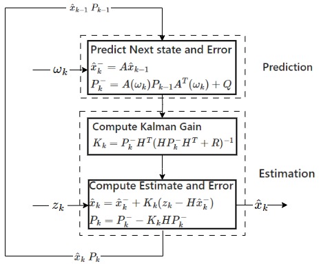
Fig. 18 Kalman filter block diagram specific to attitude determination.

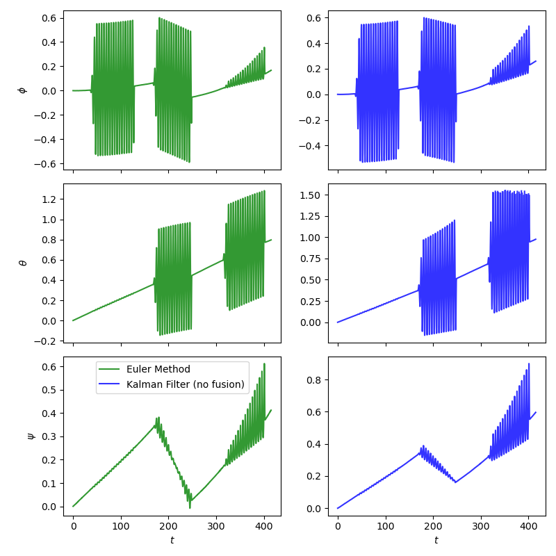
Fig. 19 The euler method for calculating attitude alongside the kalman filtered example discussed above. View in Github

This kalman filter example hasn’t improved the fit. The integration drift hasn’t been corrected for. This is because the measurement in this case didn’t contain any corrective information so didn’t correct for drift. The only difference the kalman filter makes in this case is it puts a greater emphasis on previous measurements. A better choice would be to use a sensor which doesn’t rely on the previous measurement to calculate attitude.

5.3 Kalman filters with sensor fusion

Sensor fusion involves combining different sensors to get a better estimate. A typical six axis IMU will contain a gyroscope and an accelerometer. Accelerometer data to calculate attitude but is noisier than gyroscope data. However accelerometer data can be used to calculate attitude without drift as it doesn’t involve numerical integration. The aim of this part is to use the kalman filter to do sensor fusion to produce a filtered signal with less noise than the accelerometer and no drift.

Accelerometer Data

Here accelerometer data is used to calculate \(\boldsymbol{z}_k\) which represents the attitude in terms of euler parameters as measured using the accelerometer. The accelerometer measures the acceleration, \(\boldsymbol{a}\) in the x, y and z directions. A accelerometer moving at a constant velocity can always identify which direction is down due to the acceleration from gravity. This means it can determine \(\theta\) and \(\phi\) but not \(\psi\).

The acceleration in the body fixed frame, the frame of the craft as seen by a stationary observer on earth is given by:

Where \(\boldsymbol{g} = \begin{bmatrix} 0 \\ 0 \\ g \end{bmatrix}\)

(47)\[[\boldsymbol{a}]_B = [\dot{\boldsymbol{v}}]_B - [\boldsymbol{g}]_B\]

Where \(\dot{\boldsymbol{v}}\) is the translational acceleration and \(\boldsymbol{g}\) is the acceleration due to gravity. Assumption: the translational acceleration of the body is zero and the accelerometer is located at the center of rotation for this example.

Note

B is the linear transformation matrix which transforms form the frame of the earth to the frame of the device.

\[\begin{split}B = \begin{bmatrix} \cos \psi \cos \theta & \sin \psi \cos \theta & -\sin \theta \\ \cos \psi \sin \theta \sin \phi - \cos \phi \sin \psi & \sin \psi \sin \theta \sin \phi + \cos \phi \cos \psi & \cos \theta \sin \phi \\ \cos \psi \sin \theta \cos \phi + \sin \phi \sin \psi & \sin \psi \sin \theta \cos \phi - \sin \phi \cos \psi & \cos \theta \cos \phi \end{bmatrix} \end{split}\]

This can be written in terms of unit vectors describing the effects on the \(x\), \(y\) and \(z\) components.

\[B = \begin{bmatrix} \hat{\boldsymbol{n}}_x & \hat{\boldsymbol{n}}_y & \hat{\boldsymbol{n}}_z \end{bmatrix}\]

where \(\hat{n}_x\), \(\hat{n}_y\) and \(\hat{n}_z\) are 3 dimensional unit vectors in the \(x\), \(y\) and \(z\) directions.

The acceleration in the frame of the body can be calculated from its position relative to the earth:

(48)\[\begin{split}[\boldsymbol{a}]_B = - B\boldsymbol{g} = - g \hat{\boldsymbol{n}}_z = g \begin{bmatrix} \sin{\theta} \\ -\cos{\theta}\sin{\phi} \\ -\cos{\theta}\cos{\phi} \end{bmatrix}\end{split}\]

In component form \(\boldsymbol{a} = \begin{bmatrix} a_1 \\ a_2 \\ a_3 \end{bmatrix}\) rearranging (48) gets:

(49)\[\theta = \arcsin(\frac{a_1}{g}) \quad \phi = \arcsin(\frac{-a_2}{g\cos{\theta}})\]

From the accelerometer data alone it is possible to directly calculate \(\theta\) and \(\phi\) but not \(\psi\). In this example let \(\psi = 0\) since no oscillations were performed in the \(\omega_3\) direction.

Warning

Additional noise has been added to the accelerometer readings to make the effects of the kalman filter more visible. Usually the accelerometer is more sensitive to noise than the gyroscope. Although the accelerometer data in the next few examples is definitely nosier it is hard to visualize, therefore additional gaussian noise has been added.

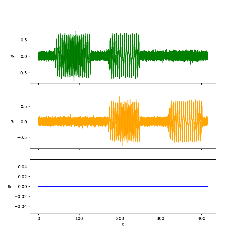
Fig. 20 yaw-pitch-roll against time using only accelerometer data for the same calibration mentioned above. View in Github

Fig. 20 is much nosier than the predicted data from the gyroscope, see Fig. 17. For small \(k\) the gyroscope is more accurate as the drift is less significant compared to the noise from the accelerometer however for large \(k\) the accelerometer is more accurate as the gyroscope measurements are subject to drift.

Improved Kalman Filter

Using the real world accelerometer and gyroscope data \(Q\) and \(R\) were tuned to obtain the optimal fit for the data.

Given quaternion components \(\boldsymbol{\beta}_0\) ( \(\beta_1\), \(\beta_2\), and \(\beta_3\)) the Euler angles ( \(\phi\), \(\theta\), \(\psi\)) can be calculated as:

\[\begin{split}\phi &= \arctan\left(\frac{2(\beta_1 \beta_2 + \beta_0 \beta_3)}{\beta_0^2 + \beta_1^2 - \beta_2^2 - \beta_3^2}\right) \\ \theta &= \arcsin\left(-2(\beta_1 \beta_3 - \beta_0 \beta_2)\right) \\ \psi &= \arctan\left(\frac{2(\beta_2 \beta_3 + \beta_0 \beta_1)}{\beta_0^2 - \beta_1^2 - \beta_2^2 + \beta_3^2}\right)\end{split}\]

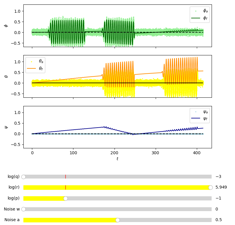
Fig. 21 Testing the kalman filter with small \(q\) and large \(r\). \(\phi_a\) represents \(\phi\) measured from accelerometer data. \(\phi_f\) represents \(\phi\) from the kalman filter with sensor fusion. View in Github

Fig. 21 is similar to the predicted data in Fig. 17 which would suggest the filter is working correctly as small \(q\) and large \(r\) mean the filter gives more weighting to predicted (gyroscope) data compared to measured (accelerometer) data.

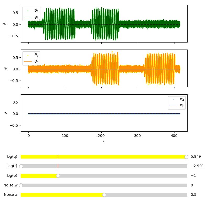
Fig. 22 Testing the kalman filter with large \(q\) and small \(r\). \(\phi_a\) represents \(\phi\) measured from accelerometer data. \(\phi_f\) represents \(\phi\) from the kalman filter with sensor fusion. View in Github

Fig. 22 is very noisy and is similar to the predicted data in Fig. 20, similarly this would suggest the filter is working correctly since large \(q\) and small \(r\) mean the filter gives more weighting to measured data compared to predicted data.

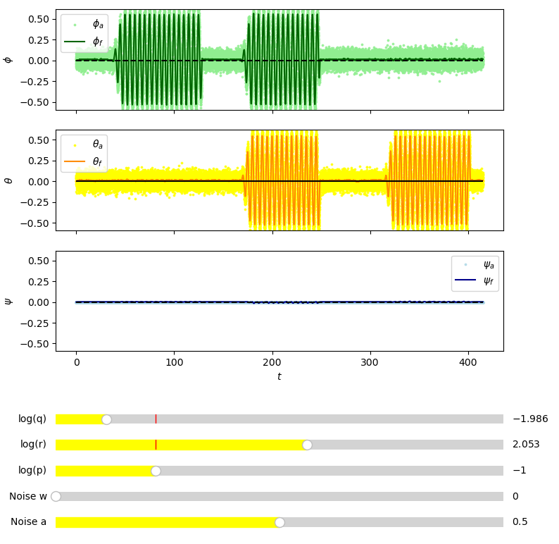
Fig. 23 Kalman filter tuned optimally by eye. \(\phi_a\) represents \(\phi\) measured from accelerometer data. \(\phi_f\) represents \(\phi\) from the kalman filter with sensor fusion. View in Github

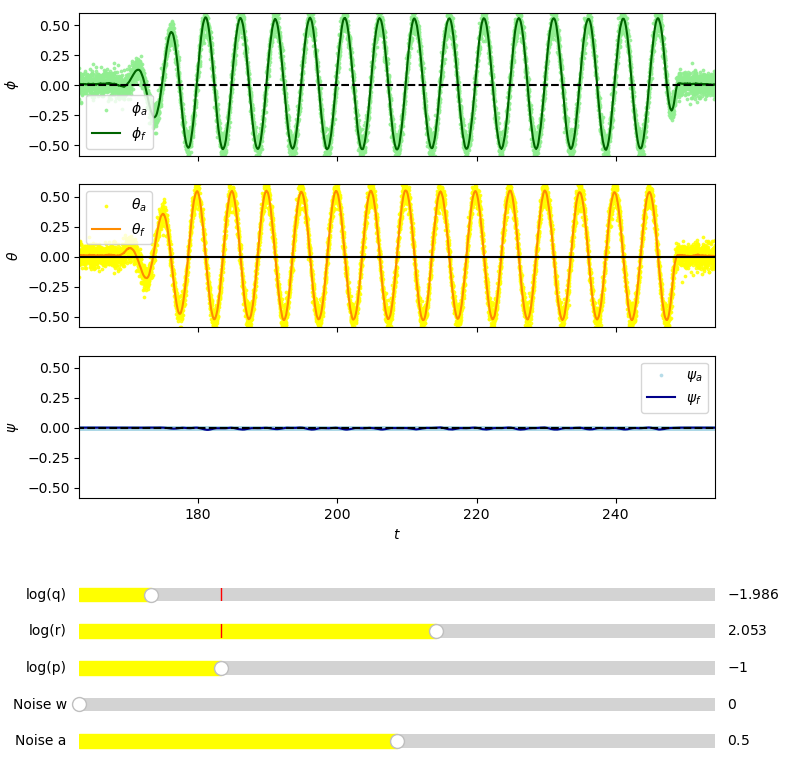
Fig. 24 Zoomed in Fig. 23. \(\phi_a\) represents \(\phi\) measured from accelerometer data. \(\phi_f\) represents \(\phi\) from the kalman filter with sensor fusion. View in Github

Fig. 23 and Fig. 24 show the kalman filter has produced a very good fit. The filtered signal appears both noise, drift and delay free.

5.4 Summary

Lets compare all three filters side by side.

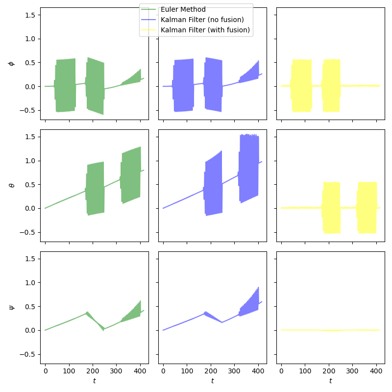
Fig. 25 All three filters side by side. View in Github

Figure Fig. 25 shows the only the kalman filter (with fusion) is accurate for determining attitude in the longrun. Even though the error from numerical integration is small if it isn’t regularly corrected for will be subject to integration drift.

The Kalman filter produced an excellent fit in this case as the prediction (from gyroscope) and measurement (from accelerometer) were complimentary to each other. The gyroscope was less susceptible to noise but was susceptible to drift whereas the accelerometer was more susceptible to noise and less susceptible to drift. Sensor fusion gets the best of both worlds.

Idea

Rewrite the part of the code that carries out kalman filter calculations and determines A in C++ as the programme runs really slowly.