2 Kalman filters

A Kalman filter compares the predicted state, \(\hat{x}^-_k\), with measurements, \(z_k\), to create an estimate of the true state, \(\hat{x}_k\). This section introduces the Kalman filter, its algorithm and why its useful.

Important

Predictions and estimates are not interchangeable when talking about Kalman filters. A prediction is a forecast of the next state based on the previous state and the mathematical model. Whereas a estimate is an update of the predicted state once new measurements have been taken.

Note

In all future sections scalars will be written as plain text \(a\) and vectors will be written in bold \(\boldsymbol{a}\). Here the symbols are context free so so are all in plain text.

2.1 Dictionary

The Kalman filter deals with the linear state model. Where the state evolves linearly according to \(A\):

(12)\[x_{k+1} = Ax_k + w_k\]

As long as no forcing function is present. The measurement can be described as:

(13)\[z_k = Hx_k + v_k \]

Where \(w_k\) and \(v_k\) are both distributed normally with mean \(0\).

A forcing function is something external that deliberately changes how the system behaves. E.g. When modelling a car rolling down a hill the cars motion is determined by gravity. Applying the cars breaks would be an example of a forcing function.**

• \(x_k\) is the actual (but unknown) state vector at time \(t_k\) e.g. the true position and velocity of a car. \(x_k\). \(n\times 1\) column vector.

• \(z_k\) is the measurement of the state from the sensor at time \(t_k\), but contains noise and errors e.g. the GPS position of the car. \(m \times 1\) column vector.

• \(A\) is the state transition matrix. \(A\) represents the “rules of motion” of the system. It describes how \(\hat{x}_k\) evolves from one time step to the next, assuming there is no external factors changing it (a forcing function). For example if you knew a cars velocity at time \(t_k\) you could use \(A\) to predict where it would be at time \(t_{k+1}\). \(n\times n\) matrix.

Note

\(A\) isn’t always a constant matrix, it can be dependent on time, or measurements from other sensors.

• \(\hat{x}_k\) and \(\hat{x}^-_k\) represent the best estimate and prediction of \(x_k\) respectively. \(\hat{x}^-_k\) is a prediction of the next state based on the physics of the system which is modeled using \(A\). \(\hat{x}_k\) is a updated estimate which blends the model based prediction \(\hat{x}^-_k\) and the measurement \(z_k\). \(\hat{x}_k\) is the end output from the Kalman filter.

• \(H\) is the state to measurement matrix. \(H\) is the translator between the system’s state and what can be measured. It explains how, if there were no noise or errors, the true state would appear in the sensor. E.g. if the model uses position to predict velocity but the sensor only measures position how \(H\) only picks out position. \(m \times n\) matrix.

• \(\hat{z}^-_k\) and \(\hat{z}_k\) is the what the model predicts and estimates the measurements should be respectively:

(14)\[ \begin{align}\begin{aligned}\hat{z}_k &= H\hat{x}_k\\\hat{z}^-_k &= H\hat{x}^-_k\end{aligned}\end{align} \]

(14) is useful for determining \(H\).

• \(w_k\) is the linear process noise vector or noise associated with the prediction. \(w_k\) is white sequence noise (random noise uncorrelated with time), which makes the models prediction imperfect. E.g. unexpected bumps in the road for a moving car. \(n \times 1\) column vector.

• \(v_k\) is the linear measurement noise vector, noise associated that corrupts \(z_k\). Even if the true state is fixed, the measurements can change due to sensor imperfections. E.g. temperature measurements using a thermometer will be slightly different each time you measure. \(m \times 1\) column vector.

• \(Q\) is the covariance matrix of \(w_k\) i.e. how much the true state is expected to deviate from the predictions made by the state transition model. Large \(Q\) assumes the measurements are more reliable than the model and puts a larger weighting on \(z_k\) compared to \(\hat{x}^-_k\) when computing \(\hat{x}_{k+1}\). Smaller \(Q\) puts more trust in the model \(\hat{x}^-_k\) compared to \(z_k\). \(n \times n\) matrix.

(15)\[Q_k = \mathbb{E}[w_k w_k^T]\]

[BH12] (chapter 4)

• \(R\) is the covariance matrix of \(v_k\). i.e. how much the measured state is effected by noise in the state transition model. \(R\) tells the Kalman filter how much to “trust” the measurements compared to model predictions. Large \(R\) suggests the model is more reliable than the measurements and puts more emphasis on \(\hat{x}^-_k\) compared to \(z_k\) when computing \(\hat{x}_{k+1}\), small \(R\) puts more emphasis on \(z_k\) compared to \(\hat{x}^-_k\). \(m \times m\) matrix.

(16)\[R_k = \mathbb{E}[v_k v_k^T]\]

[BH12] (chapter 4)

• \(e_k\) and \(e^-_k\) are the error in the estimation and the error in the prediction respectively defined as \(e_k = x_k-\hat{x}_k\) and \(e^-_k = x_k-\hat{x}^-_k\). \(n \times 1\) column vector.

• \(P_k\) and \(P^-_k\) are the associated error covariance matrices for \(e_k\) and \(e^-_k\) respectively defined by: \(n \times n\) matrix.

(17)\[P_k = \mathbb{E}[e_k e_k^T]\]

and

(18)\[P^-_k = \mathbb{E}[e^-_k (e^-_k)^T]\]

[BH12] (chapter 4)

• \(K_k\) is the Kalman gain which has similar effects to \(\alpha\) in the low pass filter. \(n \times m\) matrix. It is a blending factor that determines how much of the prediction and measurement goes into the updated estimate \(\hat{x}_k\). The Kalman gain is determined by the covariance matrices \(P^-_k\), \(H\), \(R\) and \(Q\).

• \(x_0\) is the initial state estimate. provided at the start of the estimation process.

• \(P_0\) is the initial error covariance matrix estimate.

Important

The Kalman filter parameters are the parameters set by the user before fitting the data they are: \(A\), \(Q\), \(H\), \(R\), \(\hat{x}_0\) and \(P_0\).

2.2 Estimation step

The prediction \(\hat{x}^-_k\) and measurement are combined using the blending factor \(K_k\) (yet to be determined) below to determine the updated estimate \(\hat{x}_k\).

(19)\[\hat{x}_k = \hat{x}^-_k + K_k(z_k - H\hat{x}^-_k)\]

this is known as the update step \(K_k\) determines how much of each \(z_k\) and \(\hat{x}^-_k\) goes into \(\hat{x}_k\) i.e. how much the measurement is trusted compared to the prediction.

Aside: Connection between Kalman filter and low pass filter

Equation (19) can be rewritten as:

(20)\[\hat{x}_k = (\mathbb{I} + K_k H)\hat{x}^-_k + K_k z_k\]

Letting \(H = \mathbb{I}\) and \(\alpha= 1-K_k\) a first order low pass filter is recovered similar to (7).

(21)\[\hat{x}_k = \alpha \hat{x}^-_{k} + (1 - \alpha) z_k\]

A low pass filter smooths out noisy data by blending the previous estimate with new data using a fixed weighting factor \(\alpha\). The Kalman filter automatically adjusts its version of \(\alpha\) essentially \(K_k\) to decide how to weight the previous estimate and the new data for each time step depending on how much uncertainty there is in the prediction and measurement.

The mean square error (MSE) between \(\hat{x}_k\) and \(x_k\) is the performance criterion for the Kalman filter. The MSE is related to the terms in the leading diagonal of \(P_k\). Here an expression for \(K_k\) is derived that minimizes the MSE. An expression from the definition of \(P_k\) from (17) in terms of our Kalman parameters is required. The problem is (17) contains \(e_k\) which can’t be computed since \(x_k\) is unknown.

First an expression for \(\hat{x}_k\) was determined by subbing (13) into (19), to rewrite the estimation update equation:

(22)\[\hat{x}_k = \hat{x}^-_k + K_k(Hx_k+v_k-H\hat{x}^-_k)\]

then an expression for \(P_k\) was obtained by subbing (22) into (17):

(23)\[P_k = \mathbb{E} \left\{ \left[ (x_k - \hat{x}_k^-) - K_k \left( H_k {x}_k + v_k - H_k \hat{x}_k^- \right) \right] \left[ (x_k - \hat{x}_k^-) - K_k \left( H_k {x}_k + v_k - H_k \hat{x}_k^- \right) \right]^T \right\}\]

In depth expectation simplification

By comparing (23) and (17) the estimation error \(e_k\) is built from the error in prediction and the error effect of measurement noise. The estimation error after the update step is:

(24)\[e_k = (x_k - \hat{x}_k^-) - K_k \left( H_k {x}_k + v_k - H_k \hat{x}_k^- \right)\]

Initially \(e_k\) is the error between the true state and the prediction. The Kalman gain adjusts this based on what is actually measured \(z_k = H_k {x}_k + v_k\) and what the expected measurment is \(\hat{z} = H_k \hat{x}_k^-\) based on the model. Grouping the terms more intuitively by substituting in the definition for the prediction error \(e^-_k = x_k - \hat{x}_k^-\) gets:

(25)\[e_k = e^-_k \Omega_k - K_kv_k\]

Where \(\Omega_k = I - K_k H_k\) describes how much of the prediction error remains after the update. Subbing (25) into (17) gives:

(26)\[P_k = \mathbb{E}[(e^-_k \Omega_k - K_kv_k)(e^-_k\Omega_k - K_kv_k)^T]\]

After expanding the brackets 4 terms are obtained:

(27)\[P_k = \mathbb{E}[ \Omega_k, e^-_k (e^-_k)^T \Omega_k^T - \Omega_k, e^-_k v^T K_k^T - K_k v (e^-_k)^T \Omega^T + K_k v v^T K_k^T]\]

Then using the useful identity \(\mathbb{E}[Ax + By] \equiv A\mathbb{E}[x] + B \mathbb{E}[y]\) (27) can be rewritten:

(28)\[P_k = \Omega_k, \mathbb{E}[e^-_k (e^-_k)^T] \Omega_k^T - \Omega_k \mathbb{E}[e^-_k v^T] K_k^T - K_k \mathbb{E}[v (e^-_k)^T] \Omega^T + K_k \mathbb{E}[v v^T] K_k^T\]

The first term represents the uncertainty left from the prediction after the update. The last term represents the uncertainty added by the measurement noise. The two middle terms represent the interaction between the prediction error and the measurement noise they are both zero since \(e_k\) and \(v_k\) are both have mean of \(0\) and are independent. Subbing in (18) into the first term, (16) into the last and our definition of \(\Omega_k\) term gets (29).

Performing the expectations leaves an equation for \(P_k\) in terms of Kalman filter parameters:

(29)\[P_k = (I-K_kH_k)P^-_k(I-K_kH_k)^T+K_kR_kK^T_k\]

Which is a general expression for the updated error covariance matrix for suboptimal \(K_k\). Now optimize \(K_k\) by minimizing the MSE corresponding to finding the value of \(K_k\) that minimizes the individual terms along the leading diagonal of \(P_k\) as these terms represent the estimation error variances for the elements of the state vector elements being selected. This leaves:

For a more detailed derivation see [BH12] (chapter 4).

(30)\[K_k = P^-_k H^T (H P^-_k H^T + R)^{-1}\]

In this case \(K_k\) is the optimum Kalman gain. When considering the optimum Kalman gain (29) can be simplified by ignoring the last two terms:

(31)\[P_k = P^-_k - K_k H P^-_k\]

[BH12] (chapter 4).

Whereas the low pass filter passes \(\hat{x}_{k-1}\) directly between time steps \(t_{k-1}\) and \(t_{k}\) the Kalman filter predicts the next step before a measurement is carried out and compares this with the measurement to give new estimate.

Note

\(H\) and \(R\) are only used in the prediction step.

The equations (19), (30) and (31) together describe the estimation step of the Kalman filter.

2.3 Prediction step

Unlike the low pass filter Kalman filters also consider the physics of the system, the predictions which are used alongside measurements for state estimation. The system dynamically changes over time and is modelled using \(A\), which describes how the state is predicted to change between \(t_k\) and \(t_{k+1}\):

(32)\[\hat{x}^-_{k+1} = A \hat{x}_k\]

The error covariance matrix associated with this prediction \(\hat{x}^-_{k+1}\) is obtained from:

If \(\mu_x\) is transformed linearly \(\mu_y = F\mu_x\) its covariance matrix, \(\Sigma_x\), can be transformed using \(\Sigma_y = F\Sigma_xF^T\). [BAOOl21] (chapter 2)

(33)\[P^-_k = AP_kA^T+Q\]

\(Q\) also appears here as this is how much the true state is expected to vary from the predictions. Together equations (32) and (33) equations encode the prediction phase of the filter.

Note

\(A\) and \(Q\) are only used in the prediction step.

2.4 Summary

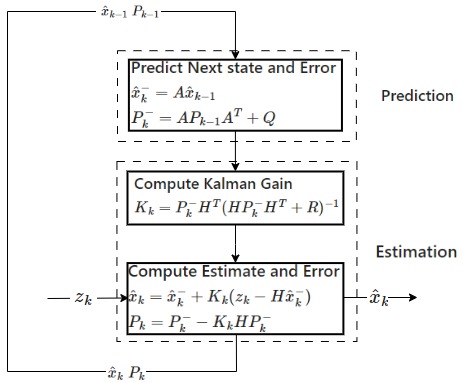
Fig. 7 Block diagram of the Kalman filter process.

• \(A\) and \(H\) are essential for the Kalman filter if these are incorrect the filter will not converge.

• \(Q\) and \(R\) are used for tuning and ensure an optimum fit.

• \(x_0\) and \(P_0\) are initial estimates the filter will still converge even if these are wrong.

• \(K_k\) and \(P_k\) are internal parameters.

• \(z_k\) are the inputs (measured state)

• \(\hat{x}_k\) are the outputs (estimated state)