3 Example: Battery output

This example looks at how a Kalman filter can be used to fit a constant signal in this case the output from a battery. The aim of this simple example is to experiment with changing the Kalman parameters \(A\), \(H\), \(Q\), \(R\), \(\hat{x}_0\) and \(P_0\). This example was inspired by Dr Shane Ross a link to the video can be found here.

3.1 Model

• \(\hat{x}_k\) is the estimate of the true battery output in volts, \(n = 1\),

• \(z_k\) is the measured battery output in volts, \(m=1\) In this very simple example \(A\), \(H\), \(Q\) and \(R\) are all scalars since \(m=n=1\)

• \(A=1\) the battery output is constant which means \(x_{k+1}\) = \(x_k\) comparing with (32) shows \(A = 1\)

• \(Q = 0\) Since the battery output is known to be constant.

• \(H = 1\) since estimate corresponds directly to measurement see (14).

• \(R = 4\) initially but was determined through tuning.

• \(x_0\) was set to 5

• \(P_0\) was set to 1

3.2 Testing

The code for this example can be found here. The code is broken up into 3 files: GenTestSig.py which generates the true signal (a constant value) and adds gaussian noise to it; SimpleKalman.py contains the algorithm for the kalman filter for the 1D case; and TestWidget.py calls functions from the other files and plots the results, with a widget so the effects of the kalman parameters can be easily visualized.

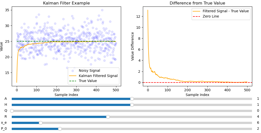
Fig. 8 Kalman filter used to fit a non-varying signal with a large amount of noise.

Fig. 8 shows that convergence is faster and smoother than the average filter. This makes sense as the kalman filter looks at both the model and the data to reduce noise.

Fig. 9 Fig. 8 but with smaller \(R\).

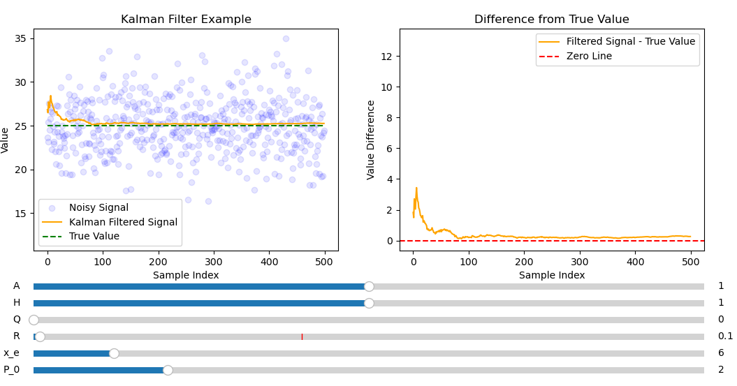
Fig. 9 shows smaller \(R\) makes convergence less smooth. This puts more faith in noisy \(z_k\) compared to less noisy \(\hat{x}^-_k\) so in the correction stage of the kalman filter more emphasis will be put on noisy \(z_k\) than on less noisy \(\hat{x}^-_k\). The signal will converge faster when \(R\) is smaller as the initial guess is far from \(x_k\), this means initially \(x^-_k\) will be less accurate than \(z_k\) since the prediction phase assumes that \(\hat{x}^-_{k} = \)\hat{x-1}_k$ which for the initial guess is incorrect. The downside of this is that the signal is more effected by noise.

Fig. 10 Fig. 8 but with larger \(R\).

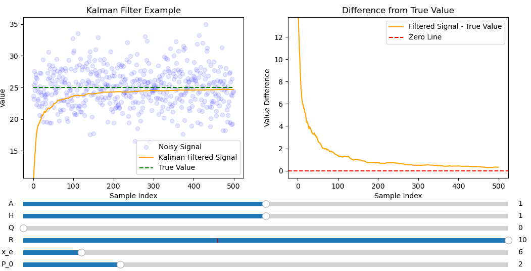
Fig. 10 shows slower convergence than figures 4.1 and 4.2 but has the smoothest convergence of the three. Fig. 8 seems to be best as it has a good tradeoff between a noise free filtered signal and fast convergence.

Fig. 11 Fig. 8 with H set to \(1.115\) rather than \(1\)

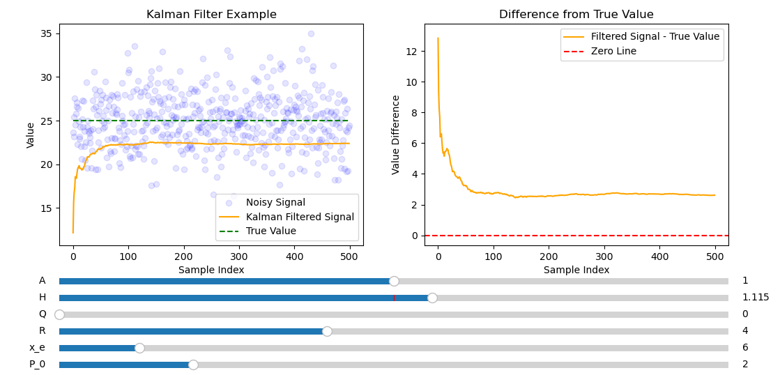
Varying \(H\) will lead to the Kalman filter converging to the wrong value since the measurement directly measures the state only satisfied by \(H = 1\).

Fig. 12 Fig. 8 with \(A\) set to 1.004 rather than 1.

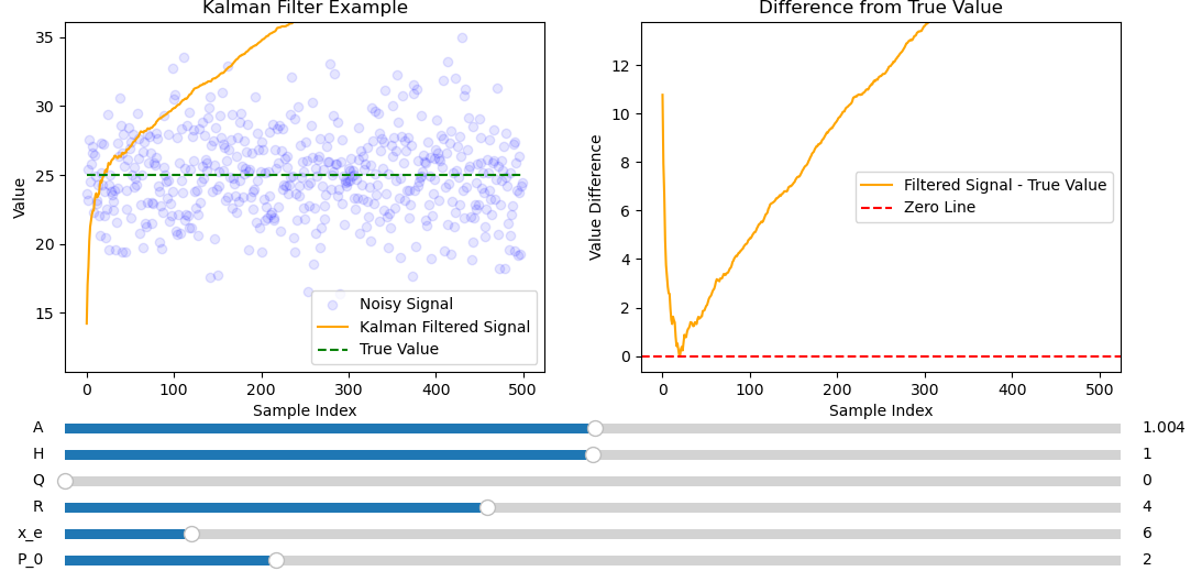
This causes the Kalman filter to diverge since only \(A=1\) describes a straight line. It diverges quickly since \(Q=0\) puts more weighting on \(\hat{x}_k\) compared to \(\hat{z_k}\).

Fig. 13 Fig. 8 except with \(Q = 0.817\) rather than 1.

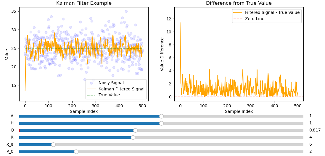
Setting \(Q\) to anything other than \(0\) in this example makes the filtered signal noisy, because it assumes the model is noisy. Increasing \(Q\) puts more trust \(\hat{z}_k\) over \(\hat{x}^-_{k}\) when predicting \(\hat{x}_k\) which means the signal becomes noisy like the data.

3.3 Summary

\(A\) describes the model and \(H\) describes how the measurement relates to the state. If these are incorrect the fit will converge to the wrong value or diverge completely. \(Q\) and \(R\) are covariance matrices, these are “tuned” to achieve optimum fit.