6 Example : Position using GPS and accelerometer data

This section improves on the the velocity from position example example by using sensor fusion. While the system using only position data (theoretically measured using GPS) works well for predicting the position, its not so good at predicting the velocity. The current model (35) represents an oversimplification as it assumes no acceleration (the acceleration doesn’t change between steps) which means that the velocity has to be corrected for by the measurements which is what causes lag. The model could be improved using real world accelerometer data which can be integrated to find velocity and position. There are other reasons for including the accelerometer data for example when GPS isn’t available due to some form of blocking e.g. being in a tunnel, the device can still roughly determine its position.

6.1 Model

Starting with the 1D case the new model is built on (35) with an additional 2nd order term:

(50)\[\begin{split}s_{k+1} &\approx s_k + \nu_k\Delta t + \frac{1}{2}a_k \Delta t^2\\ \nu_{k+1} &\approx \nu_k + a_k\Delta t\end{split}\]

The parameters from the velocity from position model remain the same, except for the model \(A\):

• \(\hat{\boldsymbol{x}}\) is the column vector of position and velocity

• \(z\) is the measurment of position from the GPS

• \(H = \begin{bmatrix} 1 & 0 \end{bmatrix}\)

• \(Q = \sigma_a^2 \begin{bmatrix} \frac{\Delta t^4}{4} & \frac{\Delta t^3}{2} \\ \frac{\Delta t^3}{2} & \Delta t^2 \end{bmatrix}\) Where \(\sigma_a\) will be the standard deviation in the acceleration measurements.

• \(R = \sigma_s^2\) Where \(\sigma_s\) will be the standard deviation in the position measurements. \(A\) needs to be a \(2 \times 2\) matrix, since it has the same number of rows and columns as the number of entries in \(\hat{z}\), but this isn’t possible since (50) contains 3 terms.

If \(\mu_x\) is transformed linearly \(\mu_y = F\mu_x\) its covariance matrix, \(\Sigma_x\), can be transformed using \(\Sigma_y = F\Sigma_xF^T\). [BAOOl21] (chapter 2)

Extended Kalman Filters

Its not possible to write the prediction stage of the kalman filter as a linear transformation. The extended kalman filter predicts the next state using:

(51)\[\hat{\boldsymbol{x}}^-_{k+1} = A\hat{\boldsymbol{x}}_k + B\boldsymbol{u}_k\]

Where \(u_k\) is the forcing function and \(B\) is its associated control matrix where \(u_k\) is the forcing function and \(B\) is its associated control matrix.

(52)\[P^-_{k+1} = A_kP_kA_k^T+B_kR^uB_k^T+Q\]

Where \(R^u\) is the associated error covariance matrix for \(u_k\). Equation (52) is the updated form of (31) with the final term \(B_kR^uB_k^T\) corresponding to the covariance update for \(R^u\). \(R^u\) becomes one of our kalman parameters when using the extended kalman filter.

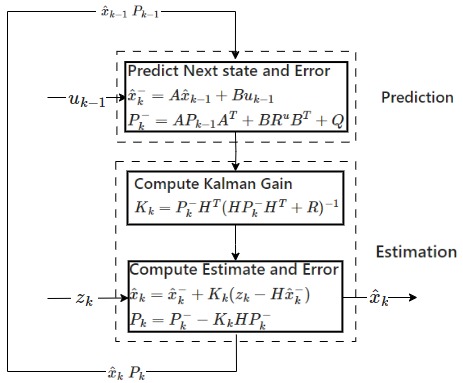
Fig. 26 Block diagram for the extended kalman filter. The estimation phase is equivalent to Fig. 7 but the prediction stage has been updated.

So (50) was rewritten in the form of (52) to determine \(u_k\) and \(B\).

\[\begin{split}\begin{bmatrix} s \\ \nu \end{bmatrix}^-_{k+1} = \begin{bmatrix} 1 & \Delta t \\ 0 & 1 \end{bmatrix} \begin{bmatrix} s \\ \nu \end{bmatrix}_k + \begin{bmatrix} \frac{1}{2} \Delta t^2 \\ \Delta t \end{bmatrix} a_k.\end{split}\]

Which gives \(u_k = \begin{bmatrix} \frac{1}{2} \Delta t^2 \\ \Delta t \end{bmatrix}\) and \(u_k = a_k\). The tuning parameter will be \(R^u = \sigma_a'^2\) determine by tuning.

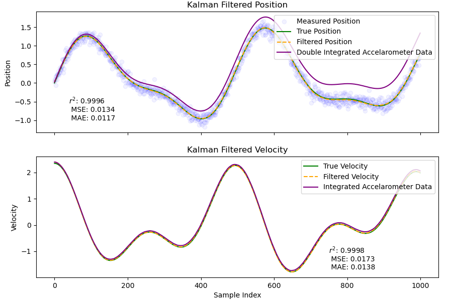
Fig. 27 Velocity and position as a function of time plotted for the extended kalman filter using the same parameters in Fig. 15, tuned by eye. View in Github

Compared to Fig. 15 the extended kalman filter with acceleration measurements gives a better fit for position and a significantly better fit for velocity, helped by the significantly better model. Even without measurement corrections the accelerometer gives a surprisingly good fit although there is a tiny bit of drift visible at the end. However the drift is significantly larger when integrated twice.

6.2 Smartphone experiment

Warning

Incomplete section. It is left here as a placeholder for future work. The experiment would have involved using kalman filters to determine the real world position and velocity of a smartphone using accelerometer and GPS data. This would have needed to consider the GPS and accelerometer having different sampling rates and noise characteristics.