4 Example: Velocity from position

This example looks at applying a Kalman filter to estimate the true position and velocity from noisy position data. This example was inspired by Dr Shane Ross a link to the videos are here: Video 1 and Video 2.

4.1 Model

In this case \(\hat{\boldsymbol{x}}_k = \begin{bmatrix} s_k \\ \nu_k \end{bmatrix}\) where \(s_k\) and \(\nu_k\) are the position and velocity (in the same direction) respectively at time \(t_k\). The correction measurement is position therefore \(z_k = s_k\). The measurement and the state are related by (14) from this \(H\) can be calculated.

(34)\[\begin{split}z_k &= H \begin{bmatrix} s_k \\ \nu_k \end{bmatrix} \\ \implies H &= \begin{bmatrix} 1 & 0 \end{bmatrix}\end{split}\]

For simplicity and to avoid needing to use a forcing function the model assumes no acceleration. The equations of motion are:

(35)\[\begin{split}s_{k+1} &\approx s_k + \nu_k\Delta t \\ \nu_{k+1} &\approx \nu_k\end{split}\]

why use \(\approx\) not \(=\)

There is a small error associated with discretizing \(dt\) since \(\Delta t\) isn’t infinitesimally small. This is negligible term to term but over a large number of terms such as in this example the error accumulates and causes drift.

Where \(\Delta t = t_{k+1} - t_k\). Now writing the update equations in matrix form the following are obtained:

(36)\[\begin{split}\begin{bmatrix} s \\ \nu \end{bmatrix}^-_{k+1} = \begin{bmatrix} 1 & \Delta t \\ 0 & 1 \end{bmatrix} \begin{bmatrix} s \\ \nu \end{bmatrix}_k\end{split}\]

\(Q\) is more complicated to calculate and is going to be a \(2 \times 2\) matrix of the form below:

\[\begin{split}Q = E[w_kw_k^T] = \begin{bmatrix} VAR(s) & COV(s,\nu) \\ COV(\nu,s) & VAR(\nu) \end{bmatrix} = \sigma_Q^2 \begin{bmatrix} \frac{\Delta t^4}{4} & \frac{\Delta t^3}{2} \\ \frac{\Delta t^3}{2} & \Delta t^2 \end{bmatrix} \end{split}\]

[BAOOl21] (chapter 2.3) [BAOOl21] (chapter 10.2) where \(\sigma_Q^2\) is the variance in the true acceleration, which is the model assumes is zero. \(\sigma_Q^2\) will be used as a tuning parameter. \(R = VAR(z_k)\) is going to be the variance in the measurements of the position which will be denoted as \(\sigma_R\) [BAOOl21] (chapter 10).

The following parameters will be used for the Kalman filter.

• \(\hat{\boldsymbol{x}}_k = \begin{bmatrix} s_k \\ \nu_k \end{bmatrix}\)

• \(z_k = s_k\)

• \(A = \begin{bmatrix} 1 & \Delta t \\ 0 & 1 \end{bmatrix}\)

• \(H = \begin{bmatrix} 1 & 0 \end{bmatrix}\)

• \(Q\) and \(R\) will are tuned using the parameters \(\sigma_a\) and \(\sigma_s\).

• \(\boldsymbol{\hat{x}}_0 = \boldsymbol{0}\) and \(P_0 \approx \begin{bmatrix} P_s & 0 \\ 0 & P_v\end{bmatrix}\) initially, these don’t matter so much as the Kalman filter will eventually find the correct values as \(k\) increases.

Note

While optimal \(P_0\) isn’t necessarily always diagonal matrix this is a good enough initial approximation as the kalman filter will converge if \(A\) and \(H\) are correct.

4.2 Implementation

The code for this example can be found here. The code is broken up into 3 files: GenTestSig.py which generates the true signal (a combination of sine waves of different frequencies) and adds gaussian noise to it; AdvKalman.py contains the algorithm for the Kalman filter for the multidimensional case; and TestUpdated.py calls functions from the other files and plots the results, with a widget so the effects of the Kalman parameters can be easily visualized.

The true signal in the graphs below is generated using a combination of \(\sin\) waves of varying amplitudes and speeds, the velocity version is the analytical derivative of this. The signal the Kalman filter is being used to fit is generated by adding random noise to the true signal and its analytical derivative. The Kalman filter is applied to the noisy position data and outputs the filtered position data and filtered velocity data. Which are graphed below. The \(r^2\) value, mean squared error (MSE) and mean absolute error (MAE) are given for both velocity and position.

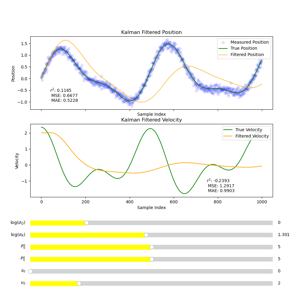
Fig. 14 Filtered, unfiltered and true position and velocity plotted against index.

In both cases the kalman filtered fit is lagging behind the true and noisy signal. This is because too much emphasis is being put on the predicted values which assumes that velocity stays the same. The true signal shows this clearly this isn’t the case. This means the velocity prediction is consistently delayed so the position will also be delayed. Since the model is erroneous it was assumed that \(w_k\) was larger and therefore \(\sigma_Q\) should be increased. A similar effect can be achieved by assuming smaller measurement noise (smaller \(v_k\)) therefore \(\sigma_R\) should be decreased.

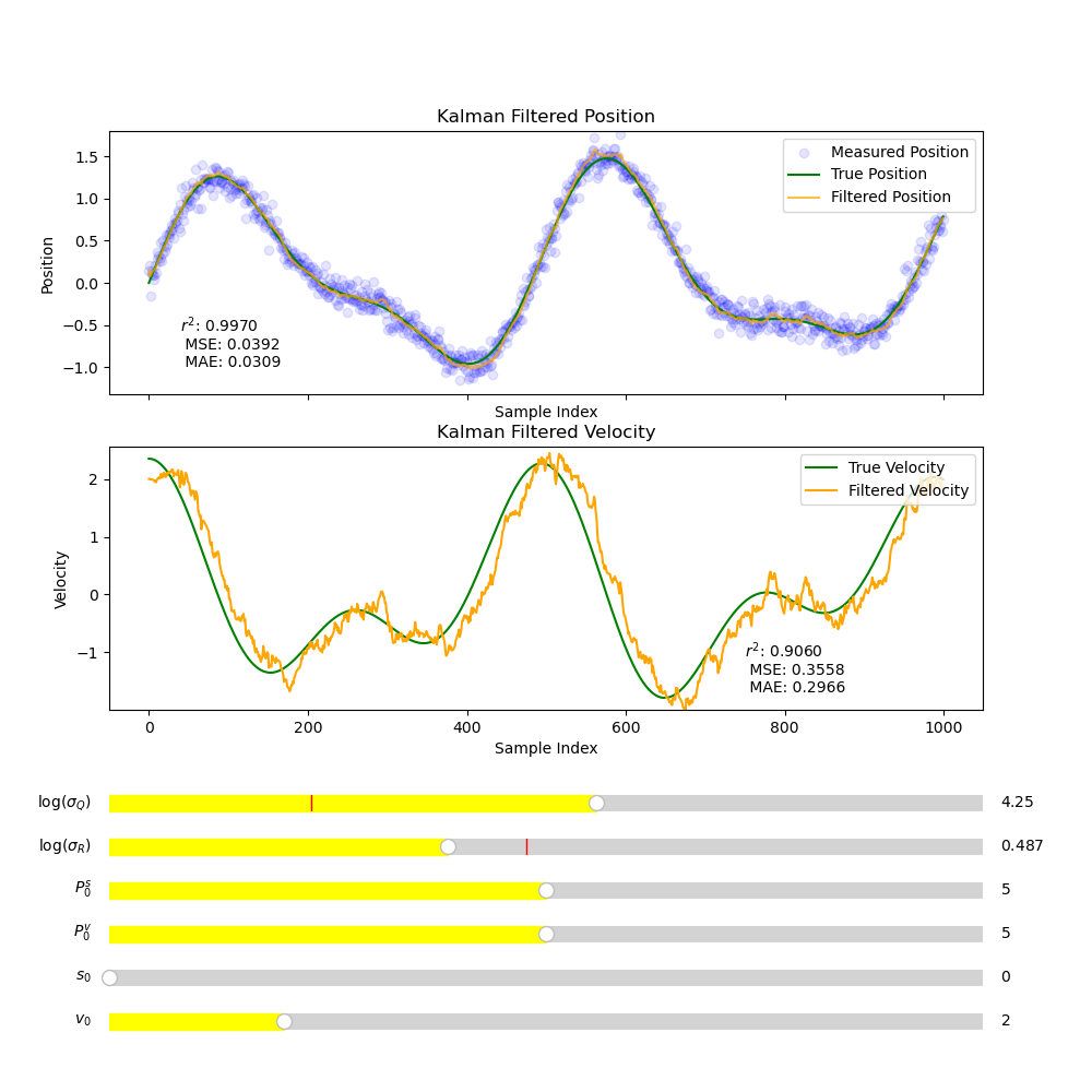
Fig. 15 See Fig. 14 with increased \(\sigma_Q\) and decreased \(\sigma_R\).

Figure Fig. 15 shows a slightly improved fit with position and a significantly improved fit with velocity. This makes sense for the position data since decreasing \(R\) increases the weighting for the measurement. However the velocity fit is now significantly less smooth since more emphasis is being put on the measured positions which is always nosier than the prediction. There is a clear tradeoff between having a a smooth fit and having an accurate fit. Smoother fits more accurately represent the true shape of the data, but will often result often this comes with drift.

Important

If the Kalman filter fit is too noisy, due to an over emphasis on \(\hat{z}_k\) compared to \(\hat{x}^-_k\) to calculate \(\hat{x}_{k}\) increasing \(R\) or decreasing \(Q\) will make the fit smoother. If the Kalman filter fit is delayed increasing \(Q\) or decreasing \(R\) will reduce the delay. Increasing \(Q\) has a similar effect to decreasing \(R\).

4.3 Summary

The kalman filter does a good job of estimating the true position from the data and the model. The velocity fit is less accurate and significantly delayed, but is good considering there are no measurements for the velocity. The fit for velocity would be greatly improved using an additional sensor to easily measure velocity or acceleration to be used in the prediction step.